Free energy implementation
For free energy calculations, there are two things that must be specified; the end states, and the pathway connecting the end states. The end states can be specified in two ways. The most straightforward is through the specification of end states in the topology file. Most potential forms support both an \(A\) state and a \(B\) state. Whenever both states are specified, the \(A\) state corresponds to the initial free energy state, and the \(B\) state corresponds to the final state.
In some cases, the end state can also be defined in some cases without
altering the topology, solely through the mdp file,
through the use of the
couple-moltype,
couple-lambda0,
couple-lambda1, and couple-intramol mdp
keywords. Any molecule type selected in couple-moltype
will automatically have a \(B\) state implicitly constructed (and
the \(A\) state redefined) according to the
couple-lambda keywords. couple-lambda0
and couple-lambda1 define the non-bonded parameters that
are present in the \(A\) state (couple-lambda0) and
the \(B\) state (couple-lambda1). The choices are
q,
vdw, and vdw-q; these indicate the Coulombic, van der Waals, or
both parameters that are turned on in the respective state.
Once the end states are defined, then the path between the end states has to be defined. This path is defined solely in the .mdp file. Starting in 4.6, \(\lambda\) is a vector of components, with Coulombic, van der Waals, bonded, restraint, and mass components all able to be adjusted independently. This makes it possible to turn off the Coulombic term linearly, and then the van der Waals using soft core, all in the same simulation. This is especially useful for replica exchange or expanded ensemble simulations, where it is important to sample all the way from interacting to non-interacting states in the same simulation to improve sampling.
fep-lambdas is the default array of \(\lambda\)
values ranging from 0 to 1. All of the other lambda arrays use the
values in this array if they are not specified. The previous behavior,
where the pathway is controlled by a single \(\lambda\) variable,
can be preserved by using only fep-lambdas to define the
pathway.

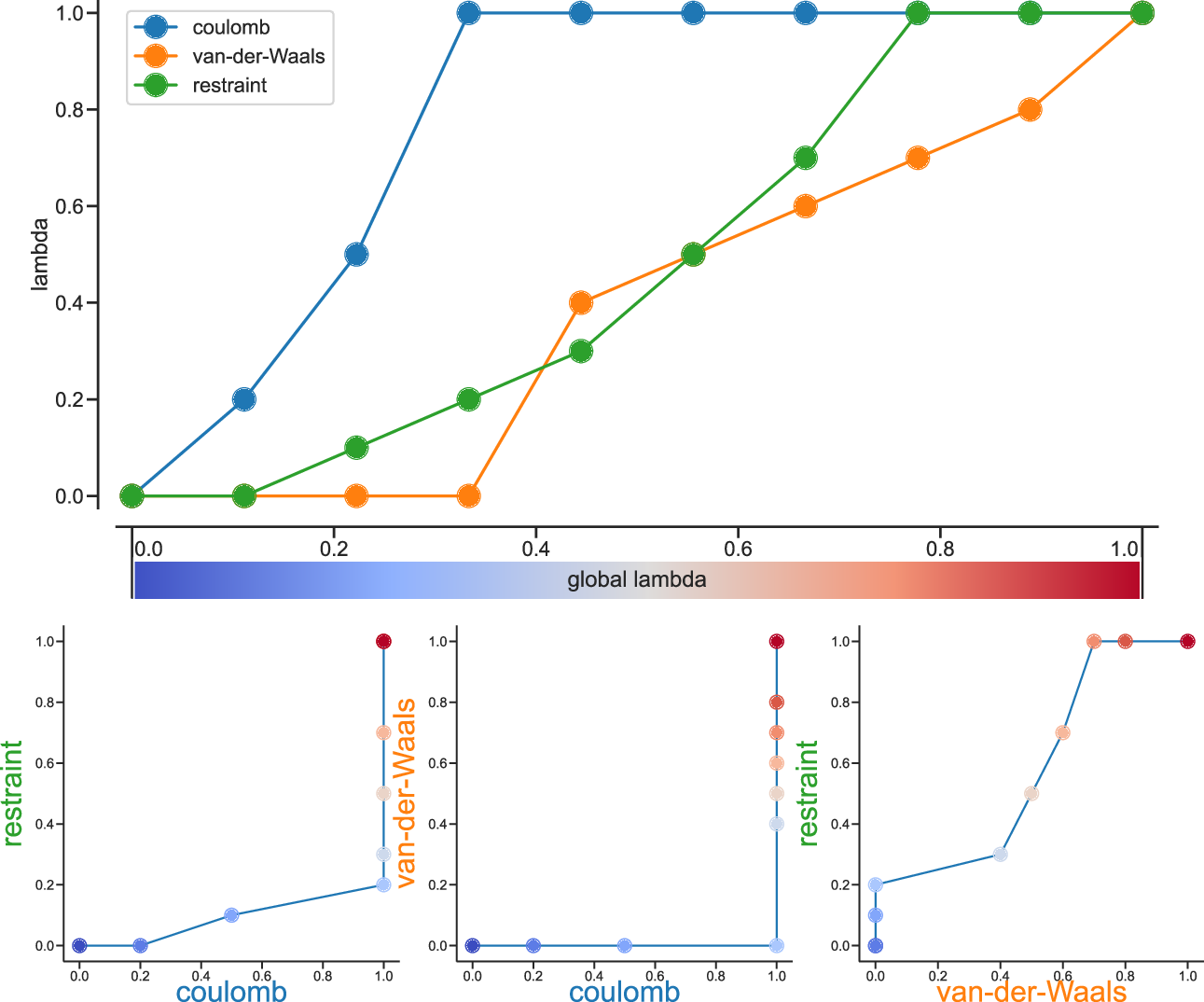
Fig. 37 Separate \(\lambda\) values for Coulomb, van-der-Waals and restraint interactions.
Fig. 37 shows an example of different lambda arrays. There, first the Coulombic terms are reduced, then the van der Waals terms, changing bonded at the same time rate as the van der Waals, but changing the restraints throughout the first two-thirds of the simulation. The corresponding \(\lambda\) vector is given here:
coul-lambdas           = 0.0 0.2 0.5 1.0 1.0 1.0 1.0 1.0 1.0 1.0
vdw-lambdas            = 0.0 0.0 0.0 0.0 0.4 0.5 0.6 0.7 0.8 1.0
bonded-lambdas         = 0.0 0.0 0.0 0.0 0.4 0.5 0.6 0.7 0.8 1.0
restraint-lambdas      = 0.0 0.0 0.1 0.2 0.3 0.5 0.7 1.0 1.0 1.0
This is also equivalent to:
fep-lambdas            = 0.0 0.0 0.0 0.0 0.4 0.5 0.6 0.7 0.8 1.0
coul-lambdas           = 0.0 0.2 0.5 1.0 1.0 1.0 1.0 1.0 1.0 1.0
restraint-lambdas      = 0.0 0.0 0.1 0.2 0.3 0.5 0.7 1.0 1.0 1.0
The fep-lambda array, in this case, is being used as the
default to fill in the bonded and van der Waals \(\lambda\) arrays.
Usually, it’s best to fill in all arrays explicitly, just to make sure
things are properly assigned.
If you want to turn on only restraints going from \(A\) to \(B\), then it would be:
restraint-lambdas = 0.0 0.1 0.2 0.4 0.6 1.0
and all of the other components of the \(\lambda\) vector would be left in the \(A\) state.
To compute free energies with a vector \(\lambda\) using thermodynamic integration, then the TI equation becomes vector equation:
or for finite differences:
The external pymbar script
can compute this integral automatically
from the GROMACS dhdl.xvg output.
Potential of mean force
A potential of mean force (PMF) is a potential that is obtained by integrating the mean force from an ensemble of configurations. In GROMACS, there are several different methods to calculate the mean force. Each method has its limitations, which are listed below.
pull code: between the centers of mass of molecules or groups of molecules.
AWH code: currently acts on coordinates provided by the pull code or the free-energy lambda parameter.
free-energy code with harmonic bonds or constraints: between single atoms.
free-energy code with position restraints: changing the conformation of a relatively immobile group of atoms.
pull code in limited cases: between groups of atoms that are part of a larger molecule for which the bonds are constrained with SHAKE or LINCS. If the pull group if relatively large, the pull code can be used.
The pull and free-energy code a described in more detail in the following two sections.
Entropic effects
When a distance between two atoms or the centers of mass of two groups is constrained or restrained, there will be a purely entropic contribution to the PMF due to the rotation of the two groups 134. For a system of two non-interacting masses the potential of mean force is:
where \(n_c\) is the number of dimensions in which the constraint works (i.e. \(n_c=3\) for a normal constraint and \(n_c=1\) when only the \(z\)-direction is constrained). Whether one needs to correct for this contribution depends on what the PMF should represent. When one wants to pull a substrate into a protein, this entropic term indeed contributes to the work to get the substrate into the protein. But when calculating a PMF between two solutes in a solvent, for the purpose of simulating without solvent, the entropic contribution should be removed. Note that this term can be significant; when at 300K the distance is halved, the contribution is 3.5 kJ mol\(^{-1}\).