Periodic boundary conditions
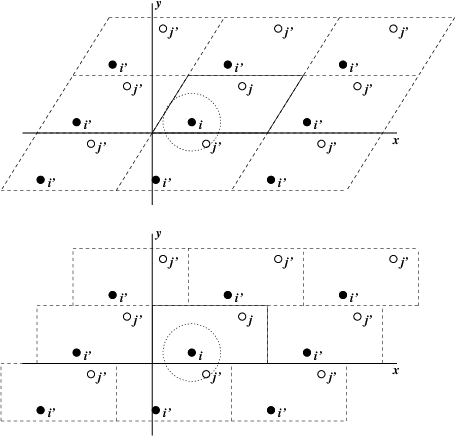
Fig. 1 Periodic boundary conditions in two dimensions.
The classical way to minimize edge effects in a finite system is to apply periodic boundary conditions. The atoms of the system to be simulated are put into a space-filling box, which is surrounded by translated copies of itself (Fig. 1). Thus there are no boundaries of the system; the artifact caused by unwanted boundaries in an isolated cluster is now replaced by the artifact of periodic conditions. If the system is crystalline, such boundary conditions are desired (although motions are naturally restricted to periodic motions with wavelengths fitting into the box). If one wishes to simulate non-periodic systems, such as liquids or solutions, the periodicity by itself causes errors. The errors can be evaluated by comparing various system sizes; they are expected to be less severe than the errors resulting from an unnatural boundary with vacuum.
There are several possible shapes for space-filling unit cells. Some, like the rhombic dodecahedron and the truncated octahedron 20 are closer to being a sphere than a cube is, and are therefore better suited to the study of an approximately spherical macromolecule in solution, since fewer solvent molecules are required to fill the box given a minimum distance between macromolecular images. At the same time, rhombic dodecahedra and truncated octahedra are special cases of triclinic unit cells; the most general space-filling unit cells that comprise all possible space-filling shapes 21. For this reason, GROMACS is based on the triclinic unit cell.
GROMACS uses periodic boundary conditions, combined with the minimum image convention: only one – the nearest – image of each particle is considered for short-range non-bonded interaction terms. For long-range electrostatic interactions this is not always accurate enough, and GROMACS therefore also incorporates lattice sum methods such as Ewald Sum, PME and PPPM.
GROMACS supports triclinic boxes of any shape. The simulation box (unit cell) is defined by the 3 box vectors \({\bf a}\),\({\bf b}\) and \({\bf c}\). The box vectors must satisfy the following conditions:
Equations (10) can always be satisfied by rotating the box. Inequalities ((11)) and ((12)) can always be satisfied by adding and subtracting box vectors.
Even when simulating using a triclinic box, GROMACS always keeps the particles in a brick-shaped volume for efficiency, as illustrated in Fig. 1 for a 2-dimensional system. Therefore, from the output trajectory it might seem that the simulation was done in a rectangular box. The program trjconv can be used to convert the trajectory to a different unit-cell representation.
It is also possible to simulate without periodic boundary conditions, but it is usually more efficient to simulate an isolated cluster of molecules in a large periodic box, since fast grid searching can only be used in a periodic system.
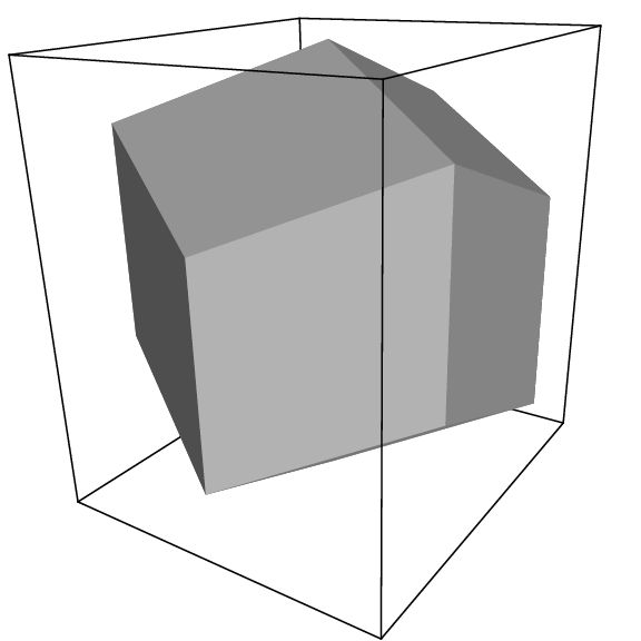
Fig. 2 A rhombic dodecahedron (arbitrary orientation).
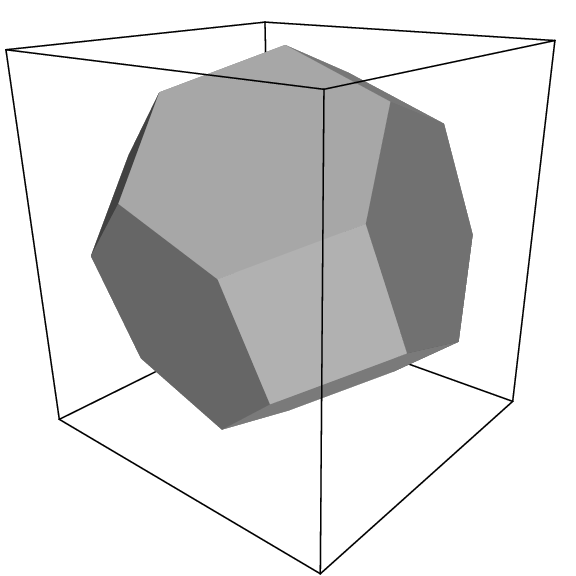
Fig. 3 A truncated octahedron (arbitrary orientation).
Some useful box types
box type |
image distance |
box volume |
box vectors |
box vector angles |
||||
|---|---|---|---|---|---|---|---|---|
a |
b |
c |
\(\angle\) bc |
\(\angle\) ac |
\(\angle\) ab |
|||
cubic |
\(d\) |
\(d^{3}\) |
\(d\) |
0 |
0 |
\(90^\circ\) |
\(90^\circ\) |
\(90^\circ\) |
0 |
\(d\) |
0 |
||||||
0 |
0 |
\(d\) |
||||||
rhombic dodcahdron (xy-square) |
\(d\) |
\(\frac{1}{2}\sqrt{2}~d^{3}\) \(0.707~d^{3}\) |
\(d\) |
0 |
\(\frac{1}{2}~d\) |
\(60^\circ\) |
\(60^\circ\) |
\(60^\circ\) |
0 |
\(d\) |
\(\frac{1}{2}~d\) |
||||||
0 |
0 |
\(\frac{1}{2}\sqrt{2}~d\) |
||||||
rhombic dodcahdron (xy- hexagon) |
\(d\) |
\(\frac{1}{2}\sqrt{2}~d^{3}\) \(0.707~d^{3}\) |
\(d\) |
\(\frac{1}{2}~d\) |
\(\frac{1}{2}~d\) |
\(60^\circ\) |
\(60^\circ\) |
\(60^\circ\) |
0 |
\(\frac{1}{2}\sqrt{3}~d\) |
\(\frac{1}{6}\sqrt{3}~d\) |
||||||
0 |
0 |
\(\frac{1}{3}\sqrt{6}~d\) |
||||||
truncated octahedron |
\(d\) |
\(\frac{4}{9}\sqrt{3}~d^{3}\) \(0.770~d^{3}\) |
\(d\) |
\(\frac{1}{3}~d\) |
\(-\frac{1}{3}~d\) |
\(71.53^\circ\) |
\(109.47^\circ\) |
\(71.53^\circ\) |
0 |
\(\frac{2}{3}\sqrt{2}~d\) |
\(\frac{1}{3}\sqrt{2}~d\) |
||||||
0 |
0 |
\(\frac{1}{3}\sqrt{6}~d\) |
||||||
The three most useful box types for simulations of solvated systems are described in Table 6. The rhombic dodecahedron (Fig. 2) is the smallest and most regular space-filling unit cell. Each of the 12 image cells is at the same distance. The volume is 71% of the volume of a cube having the same image distance. This saves about 29% of CPU-time when simulating a spherical or flexible molecule in solvent. There are two different orientations of a rhombic dodecahedron that satisfy equations (10), (11) and (12). The program editconf produces the orientation which has a square intersection with the xy-plane. This orientation was chosen because the first two box vectors coincide with the x and y-axis, which is easier to comprehend. The other orientation can be useful for simulations of membrane proteins. In this case the cross-section with the xy-plane is a hexagon, which has an area which is 14% smaller than the area of a square with the same image distance. The height of the box (\(c_z\)) should be changed to obtain an optimal spacing. This box shape not only saves CPU time, it also results in a more uniform arrangement of the proteins.
Cut-off restrictions
The minimum image convention implies that the cut-off radius used to truncate non-bonded interactions may not exceed half the shortest box vector:
because otherwise more than one image would be within the cut-off distance of the force. When a macromolecule, such as a protein, is studied in solution, this restriction alone is not sufficient: in principle, a single solvent molecule should not be able to ‘see’ both sides of the macromolecule. This means that the length of each box vector must exceed the length of the macromolecule in the direction of that edge plus two times the cut-off radius \(R_c\). It is, however, common to compromise in this respect, and make the solvent layer somewhat smaller in order to reduce the computational cost. For efficiency reasons the cut-off with triclinic boxes is more restricted. For grid search the extra restriction is weak:
For simple search the extra restriction is stronger:
Each unit cell (cubic, rectangular or triclinic) is surrounded by 26 translated images. A particular image can therefore always be identified by an index pointing to one of 27 translation vectors and constructed by applying a translation with the indexed vector (see Compute forces). Restriction (14) ensures that only 26 images need to be considered.