Enforced Rotation
This module can be used to enforce the rotation of a group of atoms, as e.g. a protein subunit. There are a variety of rotation potentials, among them complex ones that allow flexible adaptations of both the rotated subunit as well as the local rotation axis during the simulation. An example application can be found in ref. 145.
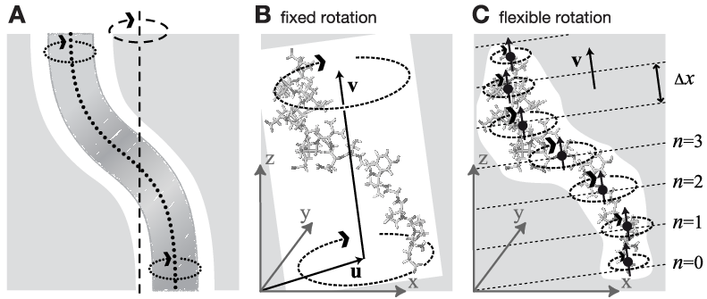
Fig. 43 Comparison of fixed and flexible axis rotation. A: Rotating the sketched shape inside the white tubular cavity can create artifacts when a fixed rotation axis (dashed) is used. More realistically, the shape would revolve like a flexible pipe-cleaner (dotted) inside the bearing (gray). B: Fixed rotation around an axis \(\mathbf{v}\) with a pivot point specified by the vector \(\mathbf{u}\). C: Subdividing the rotating fragment into slabs with separate rotation axes (\(\uparrow\)) and pivot points (\(\bullet\)) for each slab allows for flexibility. The distance between two slabs with indices \(n\) and \(n+1\) is \(\Delta x\).
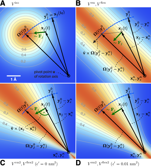
Fig. 44 Selection of different rotation potentials and definition of notation. All four potentials \(V\) (color coded) are shown for a single atom at position \(\mathbf{x}_j(t)\). A: Isotropic potential \(V^\mathrm{iso}\), B: radial motion potential \(V^\mathrm{rm}\) and flexible potential \(V^\mathrm{flex}\), C–D: radial motion2 potential \(V^\mathrm{rm2}\) and flexible2 potential \(V^\mathrm{flex2}\) for \(\epsilon'\mathrm{ = }0\mathrm{ nm}^2\) (C) and \(\epsilon'\mathrm{ = }0.01\mathrm{nm}^2\) (D). The rotation axis is perpendicular to the plane and marked by \(\otimes\). The light gray contours indicate Boltzmann factors \(e^{-V/(k_B T)}\) in the \(\mathbf{x}_j\)-plane for \(T=300\)K and \(k\mathrm{ = }200\mathrm{kJ}/(\mathrm{mol }\cdot\mathrm{nm}^2)\). The green arrow shows the direction of the force \(\mathbf{F}_{\!j}\) acting on atom \(j\); the blue dashed line indicates the motion of the reference position.
Fixed Axis Rotation
Stationary Axis with an Isotropic Potential
In the fixed axis approach (see Fig. 43 B), torque on a group of \(N\) atoms with positions \(\mathbf{x}_i\) (denoted “rotation group”) is applied by rotating a reference set of atomic positions – usually their initial positions \(\mathbf{y}_i^0\) – at a constant angular velocity \(\omega\) around an axis defined by a direction vector \(\hat{\mathbf{v}}\) and a pivot point \(\mathbf{u}\). To that aim, each atom with position \(\mathbf{x}_i\) is attracted by a “virtual spring” potential to its moving reference position \(\mathbf{y}_i = \mathbf{\Omega}(t) (\mathbf{y}_i^0 - \mathbf{u})\), where \(\mathbf{\Omega}(t)\) is a matrix that describes the rotation around the axis. In the simplest case, the “springs” are described by a harmonic potential,
with optional mass-weighted prefactors \(w_i = N \, m_i/M\) with total mass \(M = \sum_{i=1}^N m_i\). The rotation matrix \(\mathbf{\Omega}(t)\) is
where \(v_x\), \(v_y\), and \(v_z\) are the components of the normalized rotation vector \(\hat{\mathbf{v}}\), and \({\,\xi\,}:= 1-\cos(\omega t)\). As illustrated in Fig. 44 A for a single atom \(j\), the rotation matrix \(\mathbf{\Omega}(t)\) operates on the initial reference positions \(\mathbf{y}_j^0 = \mathbf{x}_j(t_0)\) of atom \(j\) at \(t=t_0\). At a later time \(t\), the reference position has rotated away from its initial place (along the blue dashed line), resulting in the force
which is directed towards the reference position.
Pivot-Free Isotropic Potential
Instead of a fixed pivot vector \(\mathbf{u}\) this potential uses the center of mass \(\mathbf{x}_c\) of the rotation group as pivot for the rotation axis,
which yields the “pivot-free” isotropic potential
with forces
Without mass-weighting, the pivot \(\mathbf{x}_c\) is the geometrical center of the group.
Parallel Motion Potential Variant
The forces generated by the isotropic potentials (eqns. (1) and (5)) also contain components parallel to the rotation axis and thereby restrain motions along the axis of either the whole rotation group (in case of \(V^\mathrm{iso}\)) or within the rotation group, in case of \(V^\mathrm{iso-pf}\).
For cases where unrestrained motion along the axis is preferred, we have implemented a “parallel motion” variant by eliminating all components parallel to the rotation axis for the potential. This is achieved by projecting the distance vectors between reference and actual positions
onto the plane perpendicular to the rotation vector,
yielding
and similarly
Pivot-Free Parallel Motion Potential
Replacing in eqn. (9) the fixed pivot \(\mathbf{u}\) by the center of mass \(\mathbf{x_c}\) yields the pivot-free variant of the parallel motion potential. With
the respective potential and forces are
Radial Motion Potential
In the above variants, the minimum of the rotation potential is either a single point at the reference position \(\mathbf{y}_i\) (for the isotropic potentials) or a single line through \(\mathbf{y}_i\) parallel to the rotation axis (for the parallel motion potentials). As a result, radial forces restrict radial motions of the atoms. The two subsequent types of rotation potentials, \(V^\mathrm{rm}\) and \(V^\mathrm{rm2}\), drastically reduce or even eliminate this effect. The first variant, \(V^\mathrm{rm}\) (Fig. 44 B), eliminates all force components parallel to the vector connecting the reference atom and the rotation axis,
with
This variant depends only on the distance \(\mathbf{p}_i \cdot (\mathbf{x}_i - \mathbf{u})\) of atom \(i\) from the plane spanned by \(\hat{\mathbf{v}}\) and \(\mathbf{\Omega}(t)(\mathbf{y}_i^0 - \mathbf{u})\). The resulting force is
Pivot-Free Radial Motion Potential
Proceeding similar to the pivot-free isotropic potential yields a pivot-free version of the above potential. With
the potential and force for the pivot-free variant of the radial motion potential read
Radial Motion 2 Alternative Potential
As seen in Fig. 44 B, the force resulting from \(V^\mathrm{rm}\) still contains a small, second-order radial component. In most cases, this perturbation is tolerable; if not, the following alternative, \(V^\mathrm{rm2}\), fully eliminates the radial contribution to the force, as depicted in Fig. 44 C,
where a small parameter \(\epsilon'\) has been introduced to avoid singularities. For \(\epsilon'\mathrm{ = }0\mathrm{nm}^2\), the equipotential planes are spanned by \(\mathbf{x}_i - \mathbf{u}\) and \(\hat{\mathbf{v}}\), yielding a force perpendicular to \(\mathbf{x}_i - \mathbf{u}\), thus not contracting or expanding structural parts that moved away from or toward the rotation axis.
Choosing a small positive \(\epsilon'\) (e.g., \(\epsilon'\mathrm{ = }0.01\mathrm{nm}^2\), Fig. 44 D) in the denominator of eqn. (20) yields a well-defined potential and continuous forces also close to the rotation axis, which is not the case for \(\epsilon'\mathrm{ = }0\mathrm{nm}^2\) (Fig. 44 C). With
the force on atom \(j\) reads
Pivot-Free Radial Motion 2 Potential
The pivot-free variant of the above potential is
With
the force on atom \(j\) reads
Flexible Axis Rotation
As sketched in Fig. 43 A–B, the rigid body behavior of the fixed axis rotation scheme is a drawback for many applications. In particular, deformations of the rotation group are suppressed when the equilibrium atom positions directly depend on the reference positions. To avoid this limitation, eqns. (18) and (23) will now be generalized towards a “flexible axis” as sketched in Fig. 43 C. This will be achieved by subdividing the rotation group into a set of equidistant slabs perpendicular to the rotation vector, and by applying a separate rotation potential to each of these slabs. Fig. 43 C shows the midplanes of the slabs as dotted straight lines and the centers as thick black dots.
To avoid discontinuities in the potential and in the forces, we define “soft slabs” by weighing the contributions of each slab \(n\) to the total potential function \(V^\mathrm{flex}\) by a Gaussian function
centered at the midplane of the \(n\)th slab. Here \(\sigma\) is the width of the Gaussian function, \(\Delta x\) the distance between adjacent slabs, and
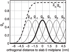
Fig. 45 Gaussian functions \(g_n\) centered at \(n \, \Delta x\) for a slab distance \(\Delta x = 1.5\) nm and \(n \geq -2\). Gaussian function \(g_0\) is highlighted in bold; the dashed line depicts the sum of the shown Gaussian functions.
A most convenient choice is \(\sigma = 0.7 \Delta x\) and
which yields a nearly constant sum, essentially independent of \(\mathbf{x}_i\) (dashed line in Fig. 45), i.e.,
with \(| \epsilon(\mathbf{x}_i) | < 1.3\cdot 10^{-4}\). This choice also implies that the individual contributions to the force from the slabs add up to unity such that no further normalization is required.
To each slab center \(\mathbf{x}_c^n\), all atoms contribute by their Gaussian-weighted (optionally also mass-weighted) position vectors \(g_n(\mathbf{x}_i) \, \mathbf{x}_i\). The instantaneous slab centers \(\mathbf{x}_c^n\) are calculated from the current positions \(\mathbf{x}_i\),
while the reference centers \(\mathbf{y}_c^n\) are calculated from the reference positions \(\mathbf{y}_i^0\),
Due to the rapid decay of \(g_n\), each slab will essentially involve contributions from atoms located within \(\approx 3\Delta x\) from the slab center only.
Flexible Axis Potential
We consider two flexible axis variants. For the first variant, the slab segmentation procedure with Gaussian weighting is applied to the radial motion potential (eqn. (18) / Fig. 44 B), yielding as the contribution of slab \(n\)
and a total potential function
Note that the global center of mass \(\mathbf{x}_c\) used in eqn. (18) is now replaced by \(\mathbf{x}_c^n\), the center of mass of the slab. With
the resulting force on atom \(j\) reads
Note that for \(V^\mathrm{flex}\), as defined, the slabs are fixed in space and so are the reference centers \(\mathbf{y}_c^n\). If during the simulation the rotation group moves too far in \(\mathbf{v}\) direction, it may enter a region where – due to the lack of nearby reference positions – no reference slab centers are defined, rendering the potential evaluation impossible. We therefore have included a slightly modified version of this potential that avoids this problem by attaching the midplane of slab \(n=0\) to the center of mass of the rotation group, yielding slabs that move with the rotation group. This is achieved by subtracting the center of mass \(\mathbf{x}_c\) of the group from the positions,
such that
To simplify the force derivation, and for efficiency reasons, we here assume \(\mathbf{x}_c\) to be constant, and thus \(\partial \mathbf{x}_c / \partial x = \partial \mathbf{x}_c / \partial y = \partial \mathbf{x}_c / \partial z = 0\). The resulting force error is small (of order \(O(1/N)\) or \(O(m_j/M)\) if mass-weighting is applied) and can therefore be tolerated. With this assumption, the forces \(\mathbf{F}^\mathrm{flex-t}\) have the same form as eqn. (35).
Flexible Axis 2 Alternative Potential
In this second variant, slab segmentation is applied to \(V^\mathrm{rm2}\) (eqn. (23)), resulting in a flexible axis potential without radial force contributions (Fig. 44 C),
With
the force on atom \(j\) reads
Applying transformation (36) yields a “translation-tolerant” version of the flexible2 potential, \(V{^\mathrm{flex2 - t}}\). Again, assuming that \(\partial \mathbf{x}_c / \partial x\), \(\partial \mathbf{x}_c / \partial y\), \(\partial \mathbf{x}_c / \partial z\) are small, the resulting equations for \(V{^\mathrm{flex2 - t}}\) and \(\mathbf{F}{^\mathrm{flex2 - t}}\) are similar to those of \(V^\mathrm{flex2}\) and \(\mathbf{F}^\mathrm{flex2}\).
Usage
To apply enforced rotation, the particles \(i\) that are to be
subjected to one of the rotation potentials are defined via index groups
rot-group0, rot-group1, etc., in the
mdp input file. The reference positions
\(\mathbf{y}_i^0\) are read from a special
trr file provided to grompp. If no such
file is found, \(\mathbf{x}_i(t=0)\) are used as
reference positions and written to trr such that they
can be used for subsequent setups. All parameters of the potentials such
as \(k\), \(\epsilon'\), etc.
(Table 16) are provided as mdp
parameters; rot-type selects the type of the potential.
The option rot-massw allows to choose whether or not to
use mass-weighted averaging. For the flexible potentials, a cutoff value
\(g_n^\mathrm{min}\) (typically \(g_n^\mathrm{min}=0.001\))
makes sure that only significant contributions to \(V\) and
\(\mathbf{F}\) are evaluated, i.e. terms with
\(g_n(\mathbf{x}) < g_n^\mathrm{min}\) are omitted.
Table 17 summarizes observables that are
written to additional output files and which are described below.
| parameter | \(k\) | \(\hat{\mathbf{v}}\) | \(\mathbf{u}\) | \(\omega\) | \({\epsilon}'\) | \({\Delta}x\) | \(g_n^\mathrm{min}\) | ||
|---|---|---|---|---|---|---|---|---|---|
| mdp input variable name | k | vec | pivot | rate | eps | slab-dist | min-gauss | ||
| unit | \(\frac{\mathrm{kJ}}{\mathrm{mol} \cdot \mathrm{nm}^2}\) | - |
nm | \(^\circ\)/ps | nm\(^2\) | nm | - |
||
| fixed axis potentials: | eqn. | ||||||||
| isotropic | V\(^\mathrm{iso}\) | (1) | x | x | x | x | - |
- |
- |
| — pivot-free | V\(^\mathrm{iso-pf}\) | (5) | x | x | - |
x | - |
- |
- |
| parallel motion | V\(^\mathrm{pm}\) | (9) | x | x | x | x | - |
- |
- |
| — pivot-free | V\(^\mathrm{pm-pf}\) | (12) | x | x | - |
x | - |
- |
- |
| radial motion | V\(^\mathrm{rm}\) | (14) | x | x | x | x | - |
- |
- |
| — pivot-free | V\(^\mathrm{rm-pf}\) | (18) | x | x | - |
x | - |
- |
- |
| radial motion 2 | V\(^\mathrm{rm2}\) | (20) | x | x | x | x | x | - |
- |
| — pivot-free | V\(^\mathrm{rm2-pf}\) | (23) | x | x | - |
x | x | - |
- |
| flexible axis potentials: | eqn. | ||||||||
| flexible | V\(^\mathrm{flex}\) | (33) | x | x | - |
x | - |
x | x |
| — transl. tol | V\(^\mathrm{flex-t}\) | (37) | x | x | - |
x | - |
x | x |
| flexible 2 | V\(^\mathrm{flex2}\) | (38) | x | x | - |
x | x | x | x |
| — transl. tol | V\(^\mathrm{flex2-t}\) | - |
x | x | - |
x | x | x | x |
| quantity | unit | equation | output file | fixed | flexible |
|---|---|---|---|---|---|
| \(V(t)\) | kJ/mol | see Table 16 | rotation |
x | x |
| \(\theta_{ \mathrm{ref}}(t)\) | degrees | \(\theta_{\mathrm{ref}}(t)=\omega t\) | rotation |
x | x |
| \(\theta_{\mathrm{av}}(t)\) | degrees | (41) | rotation |
x | - |
| \(\theta_{\mathrm{fit}}(t)\), \(\theta_{\mathrm{fit}}(t,n)\) | degrees | (43) | rotangles |
- |
x |
| \(\mathbf{y}_{0}(n)\), \(\mathbf{x}_{0}(t,n)\) | nm | (30),(31) | rotslabs |
- |
x |
| \(\tau(t)\) | kJ/mol | (44) | rotation |
x | - |
| \(\tau(t,n)\) | kJ/mol | (44) | rottorque |
- |
x |
Angle of Rotation Groups: Fixed Axis
For fixed axis rotation, the average angle \(\theta_\mathrm{av}(t)\) of the group relative to the reference group is determined via the distance-weighted angular deviation of all rotation group atoms from their reference positions,
Here, \(r_i\) is the distance of the reference position to the rotation axis, and the difference angles \(\theta_i\) are determined from the atomic positions, projected onto a plane perpendicular to the rotation axis through pivot point \(\mathbf{u}\) (see eqn. (8) for the definition of \(\perp\)),
The sign of \(\theta_\mathrm{av}\) is chosen such that \(\theta_\mathrm{av} > 0\) if the actual structure rotates ahead of the reference.
Angle of Rotation Groups: Flexible Axis
For flexible axis rotation, two outputs are provided, the angle of the entire rotation group, and separate angles for the segments in the slabs. The angle of the entire rotation group is determined by an RMSD fit of \(\mathbf{x}_i\) to the reference positions \(\mathbf{y}_i^0\) at \(t=0\), yielding \(\theta_\mathrm{fit}\) as the angle by which the reference has to be rotated around \(\hat{\mathbf{v}}\) for the optimal fit,
To determine the local angle for each slab \(n\), both reference and actual positions are weighted with the Gaussian function of slab \(n\), and \(\theta_\mathrm{fit}(t,n)\) is calculated as in eqn. (43) from the Gaussian-weighted positions.
For all angles, the mdp input option
rot-fit-method controls whether a normal RMSD fit is
performed or whether for the fit each position
\(\mathbf{x}_i\) is put at the same distance to the
rotation axis as its reference counterpart
\(\mathbf{y}_i^0\). In the latter case, the RMSD
measures only angular differences, not radial ones.
Angle Determination by Searching the Energy Minimum
Alternatively, for rot-fit-method = potential, the angle
of the rotation group is determined as the angle for which the rotation
potential energy is minimal. Therefore, the used rotation potential is
additionally evaluated for a set of angles around the current reference
angle. In this case, the rotangles.log output file
contains the values of the rotation potential at the chosen set of
angles, while rotation.xvg lists the angle with minimal
potential energy.
Torque
The torque \(\mathbf{\tau}(t)\) exerted by the rotation potential is calculated for fixed axis rotation via
where \(\mathbf{r}_i(t)\) is the distance vector from the rotation axis to \(\mathbf{x}_i(t)\) and \(\mathbf{f}_{\!i}^\perp(t)\) is the force component perpendicular to \(\mathbf{r}_i(t)\) and \(\hat{\mathbf{v}}\). For flexible axis rotation, torques \(\mathbf{\tau}_{\!n}\) are calculated for each slab using the local rotation axis of the slab and the Gaussian-weighted positions.