Electric fields
A pulsed and oscillating electric field can be applied according to:
where \(E_0\) is the field strength, the angular frequency
\(\omega = 2\pi c/\lambda\), \(t_0\) is the time
at of the peak in the field strength and \(\sigma\) is the width of
the pulse. Special cases occur when \(\sigma\) = 0 (non-pulsed
field) and for \(\omega\) is 0 (static field). See
electric-field-x for more details.
This simulated laser-pulse was applied to simulations of melting ice 146. A pulsed electric field may look ike Fig. 48. In the supporting information of that paper the impact of an applied electric field on a system under periodic boundary conditions is analyzed. It is described that the effective electric field under PBC is larger than the applied field, by a factor depending on the size of the box and the dielectric properties of molecules in the box. For a system with static dielectric properties this factor can be corrected for. But for a system where the dielectric varies over time, for example a membrane protein with a pore that opens and closes during the simulation, this way of applying an electric field is not useful. In such cases one can use the computational electrophysiology protocol described in the next section (sec. Computational Electrophysiology).
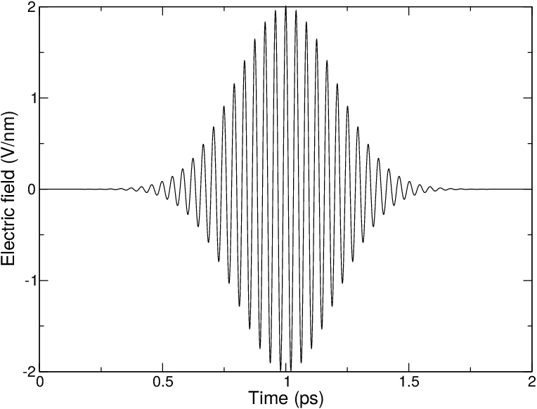
Fig. 48 A simulated laser pulse in GROMACS.
Electric fields are applied when the following options are specified in the grompp mdp file. You specify, in order, \(E_0\), \(\omega\), \(t_0\) and \(\sigma\):
electric-field-x = 0.04 0 0 0
yields a static field with \(E_0\) = 0.04 V/nm in the X-direction. In contrast,
electric-field-x = 2.0 150 5 0
yields an oscillating electric field with \(E_0\) = 2 V/nm, \(\omega\) = 150/ps and \(t_0\) = 5 ps. Finally
electric-field-x = 2.0 150 5 1
yields an pulsed-oscillating electric field with \(E_0\) = 2 V/nm,
\(\omega\) = 150/ps and \(t_0\) = 5 ps and \(\sigma\) = 1
ps. Read more in ref. 146. Note that the input file
format is changed from the undocumented older version. A figure like
Fig. 48 may be produced by passing the
-field option to gmx mdrun.