Free energy calculations
Slow-growth methods
Free energy calculations can be performed in GROMACS using a number of methods, including “slow-growth.” An example problem might be calculating the difference in free energy of binding of an inhibitor I to an enzyme E and to a mutated enzyme E\(^{\prime}\). It is not feasible with computer simulations to perform a docking calculation for such a large complex, or even releasing the inhibitor from the enzyme in a reasonable amount of computer time with reasonable accuracy. However, if we consider the free energy cycle in Fig. 9 A we can write:
If we are interested in the left-hand term we can equally well compute the right-hand term.
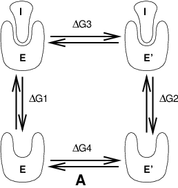
Fig. 9 Free energy cycles. A: to calculate \(\Delta G_{12}\), the free energy difference between the binding of inhibitor I to enzymes E respectively E\(^{\prime}\).
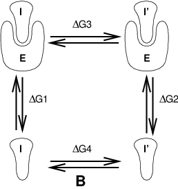
Fig. 10 Free energy cycles. B: to calculate \(\Delta G_{12}\), the free energy difference for binding of inhibitors I respectively I\(^{\prime}\) to enzyme E.
If we want to compute the difference in free energy of binding of two inhibitors I and I\(^{\prime}\) to an enzyme E (Fig. 10) we can again use (125) to compute the desired property.
Free energy differences between two molecular species can be calculated in GROMACS using the “slow-growth” method. Such free energy differences between different molecular species are physically meaningless, but they can be used to obtain meaningful quantities employing a thermodynamic cycle. The method requires a simulation during which the Hamiltonian of the system changes slowly from that describing one system (A) to that describing the other system (B). The change must be so slow that the system remains in equilibrium during the process; if that requirement is fulfilled, the change is reversible and a slow-growth simulation from B to A will yield the same results (but with a different sign) as a slow-growth simulation from A to B. This is a useful check, but the user should be aware of the danger that equality of forward and backward growth results does not guarantee correctness of the results.
The required modification of the Hamiltonian \(H\) is realized by making \(H\) a function of a coupling parameter \(\lambda: H=H(p,q;\lambda)\) in such a way that \(\lambda=0\) describes system A and \(\lambda=1\) describes system B:
In GROMACS, the functional form of the \(\lambda\)-dependence is different for the various force-field contributions and is described in section sec. Free energy interactions.
The Helmholtz free energy \(A\) is related to the partition function \(Q\) of an \(N,V,T\) ensemble, which is assumed to be the equilibrium ensemble generated by a MD simulation at constant volume and temperature. The generally more useful Gibbs free energy \(G\) is related to the partition function \(\Delta\) of an \(N,p,T\) ensemble, which is assumed to be the equilibrium ensemble generated by a MD simulation at constant pressure and temperature:
where \(\beta = 1/(k_BT)\) and \(c = (N! h^{3N})^{-1}\). These integrals over phase space cannot be evaluated from a simulation, but it is possible to evaluate the derivative with respect to \(\lambda\) as an ensemble average:
with a similar relation for \(dG/d\lambda\) in the \(N,p,T\) ensemble. The difference in free energy between A and B can be found by integrating the derivative over \(\lambda\):
If one wishes to evaluate \(G{^{\mathrm{B}}}(p,T)-G{^{\mathrm{A}}}(p,T)\), the natural choice is a constant-pressure simulation. However, this quantity can also be obtained from a slow-growth simulation at constant volume, starting with system A at pressure \(p\) and volume \(V\) and ending with system B at pressure \(p_B\), by applying the following small (but, in principle, exact) correction:
Here we omitted the constant \(T\) from the notation. This correction is roughly equal to \(-\frac{1}{2} (p{^{\mathrm{B}}}-p)\Delta V=(\Delta V)^2/(2 \kappa V)\), where \(\Delta V\) is the volume change at \(p\) and \(\kappa\) is the isothermal compressibility. This is usually small; for example, the growth of a water molecule from nothing in a bath of 1000 water molecules at constant volume would produce an additional pressure of as much as 22 bar, but a correction to the Helmholtz free energy of just -1 kJ mol\(^{-1}\). In Cartesian coordinates, the kinetic energy term in the Hamiltonian depends only on the momenta, and can be separately integrated and, in fact, removed from the equations. When masses do not change, there is no contribution from the kinetic energy at all; otherwise the integrated contribution to the free energy is \(-\frac{3}{2} k_BT \ln (m{^{\mathrm{B}}}/m{^{\mathrm{A}}})\). Note that this is only true in the absence of constraints.
Thermodynamic integration
GROMACS offers the possibility to integrate (129) or eq.
(130) in one simulation over the full range from A to B. However, if
the change is large and insufficient sampling can be expected, the user
may prefer to determine the value of \(\langle
dG/d\lambda \rangle\) accurately at a number of well-chosen intermediate
values of \(\lambda\). This can easily be done by setting the
stepsize delta_lambda to zero. Each simulation can be equilibrated
first, and a proper error estimate can be made for each value of
\(dG/d\lambda\) from the fluctuation of \(\partial H/\partial
\lambda\). The total free energy change is then determined afterward by
an appropriate numerical integration procedure.
GROMACS now also supports the use of Bennett’s Acceptance Ratio 58 for calculating values of \(\Delta\)G for transformations from state A to state B using the program gmx bar. The same data can also be used to calculate free energies using MBAR 59, though the analysis currently requires external tools from the external pymbar package.
The \(\lambda\)-dependence for the force-field contributions is described in detail in section sec. Free energy interactions.